(x/1.0574883)2.5087905)(1.5663906-0.3242146X+0.029424906X2)/(1.0),
where X=x1.55

| Examples |
|
Three examples illustrate advantages of the suggested regression method for recurrent event prediction.
Example 1.
|
| Output: |

|
Example 2. The input data for this example is generated by Monte Carlo method for Kijima model 1 with restoration factor q=0 and Weibull underlying function with shape parameter beta=2.0 and scale parameter eta=1.0. In total we had 20 components. All of them were suspended at time=4. The input file is here
|
| Output: |

|
Red solid curve in figure corresponds to the exact solution, red signs represents input data generated by simulation,
black solid curve is the regression solution. The standard deviation of obtained approximation from exact solution is also less than
the standard deviation of input data from the exact solution. The output file is here
|
|
Example 3. This example from paper [1] shows the possibility of data extrapolation using regression analysis. We consider the Kijima model with increasing restoration factor. We have simulated a statistical sample of 100 trajectories (components) from a general renewal model with the underlying Weibull distribution (scale parameter eta=1 and shape parameter beta= 2) and with Kijima I restoration factor depending on failure number, i, in the following functional form: qi = qi-1 +0.5(1- qi-1). Specifically, with q1 = 0.2, q2 = 0.6, q3 = 0.8, ... The estimation interval was truncated at 2 units of time, corresponding to ~3 failures of the system. The input file is here
|
| Output: |

|
Red curve in the figure corresponds to the exact solution. Black solid line represents obtained approximation;
dash-dotted curve is the solution obtained by Kijima model with constant restoration factor.
The example shows that by increasing the number of parameters of approximation function we can obtain better data extrapolation.
However, be advised that increasing this number can lead to overfitting phenomena. The output file is here
|
|
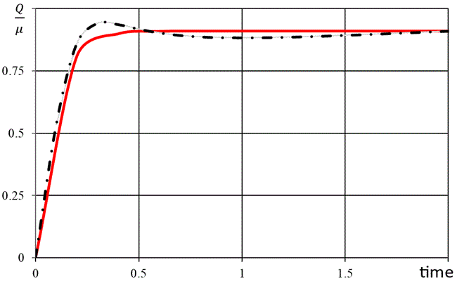
Example 4. This example shows the possibility of Unavailability Q calculation as Failure Intensity (FI) function multiplied by mean time to repair. We consider the exponential function for failure time distribution. We simulated a statistical sample of 400 trajectories (components) from a general renewal model with the underlying Weibull distribution (scale parameter eta=1 and shape parameter beta= 1). The estimation interval was truncated at 3 units of time. The input file is here
|
| Output: |

|
The result is shown by dash-dotted line.
The red curve in the figure corresponds to the exact solution.
The example shows that the model can be used for Unavailability calculation.
Note that in some cases for approximation of the derivative of the function it is required more parameters
(for example if Failure Intensity function has maximum).
|
| References |
| 1. A. Yevkin, V. Krivtsov, A generalized model for recurrent failures prediction, Reliability Engineering and System Safety 204 (2020). |
| 2. A. Yevkin, V. Krivtsov, Modeling Recurrent Failure Processes using Padé Approximants, RAMS 2025. Proceedings of Reliability and Maintainability Symposium, RAMS 2025, Florida, US. |