| General information |
| Description |
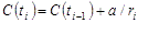
| Recurrent process (for example, failure-repair) is analyzed. First, non-parametric estimation of expected number of events is performed, then regression analysis is applied to obtained data for recurrent event prediction. To apply it, we have to calculate the cumulative intensity function (CIF) at each event time using non-parametric estimation. For this purpose we sorted all recurrence and censoring times (ages). If a recurrence age for an item is the same as its suspension age, then the recurrence time goes first. If multiple units have a common recurrence time, then they are shifted slightly, so that at any time only one event occurs. Then we calculated CIF using the following formula [1] |
|
|
|
where ri=ri-1 if ti is recurrence time, ri=ri-1-1 if ti is censoring time,
r1=N, which is the total number of items in the test.
Parameter a=1 in all cases except the case when ti corresponds to the very first failure in the test. In this case a=0.5.
This value better fits the obvious condition CIF(t)≈F(t) for small CIF (according to non-parametric estimation
for underlying failure probability function F(t)).
Note, that the accuracy of this formula significantly depends on the number of observed components. The error is in-between 1/N and 1/rN where N is the total number of components and rN is the number of operating components at the end of observation. Therefore, the formula is valid at time ti of a failure if corresponding value of CIF is much greater than 1/ri. We recommend to use this calculation only if N>10. Otherwise it is better to apply maximum likelihood estimator (MLE). However, in case of large enough number of components N, the suggested regression analysis allows better data approximation using Pade functions with many parameters and different shapes. For this reason it is also more efficient for data extrapolation (see Examples).
The main purpose of this calculation is obtaining a relatively simple formula
of data fitting y=f(x). We apply the generalized Pade functions [2] for the approximation
of data in the following form:
|
|
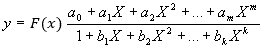
|
|
Function F(x) defines CIF for small x as CIF(x)≈F(x). It is calculated using traditional MLE
taking into account only first failures of all components assuming that the lifetime distribution is Weibull.
Having shape and scale parameters beta and eta we obtain asymptotic presentation of CIF and Weibull function
(x/eta)beta which is valid for small x. Coefficients ai, and bi should be chosen
as the best approximation of all given data. We try different values of m and k,
and different substitutions X=xq, (0.1< q ≤ 2) in the program looking for the best approximation.
As a result we obtain approximation of CIF(x) function in the entire range of argument x. Pade functions have the following advantages [2]: |
|
|
| You can find an excellent summary of properties of Pade functions here. |
| Assumptions |
| It is assumed that we have enough data for a reasonable approximation. We start to calculate the Pade function coefficients when the number of them is equal to 2, increasing this number until we reach the required accuracy or any other condition of approximation defined by user. |
| Methodology |
| If traditional method of Residual Sum of Squares (RSS) is used, the application of Pade functions in regression analysis leads to a system of nonlinear equations. This problem is resolved in our paper [3], Section 3. We have implemented this method in the suggested calculation. In addition to estimation of coefficients of rational function, it allowed us to try different combinations of m and k and apply the above mentioned substitutions X=xq. |
| Increasing the number of coefficients of approximation function from 3 until the maximum (or required accuracy) entered by user will be reached and varying the form of approximation function on each step, the program calculates and chooses the best approximation. The criterion is the standard deviation. The calculation will be completed if one of the following 2 conditions is reached: |
|
|
We suppose that this calculation would be useful to researchers and engineers looking for good approximation of data with simple formula. To check the efficiency of suggested calculation, please see examples. |
| References |
|